Wave Onset in Central Gray Matter

Details about chicken eye can be found here

[Experiment One]

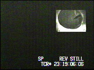
In this section we show the wave onset intrinsic optical signal as seen by two different microscopes.

Microscope1 view is shown in the inset.

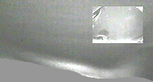
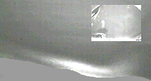
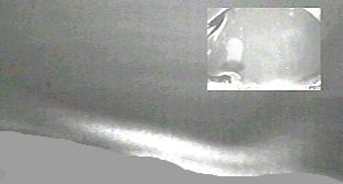
The scene is viewed from the top, the dark line is the pecten (the lenght of the pecten is about 4 mm). The illumination is made with a blue filter (450 nm, 20 nm bandwidth) set in front of an halogen lamp that provides difuse illumination.

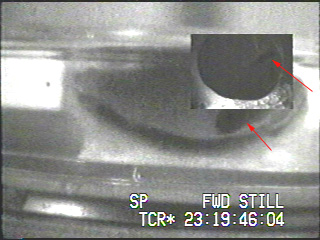A second microscope see the view from the side (90 degrees from the first one). The two arrows point the pecten as seen by the two microscopes. A red optical filter is located in front of the camera in the second microscope (625 nm, 20 nm bandwidth).

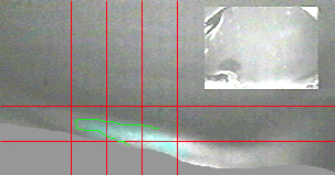
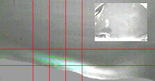
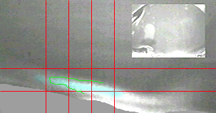
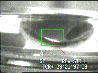A red laser beam (from a laser pointer) is focused on the retina as shown by the arrow and the green square. In the sequence shown below, the region shown in the square is amplified. This type of experimental setup was used in the sequence shown below and in the movie. More details.

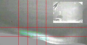
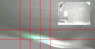
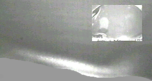
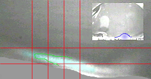
The following figure depicts the spreading depression wave onset and progression in the chicken retina during the experiment. The left column shows a sequence of snapshots of the phenomenon. The images are enhanced versions of the original ones. The .right column presents the same sequence with some markers superimposed in order to turn the wave progression easier to visualize. The images in the insets show the overall structure whereas the surrounding images are details of the small ones. See below for an explanation.

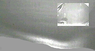
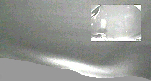
In (a) and (b) it is shown the non-stimulated state. The inset images  (a) and (b) depicts the chicken eye structures in quiescent stage. The following images show the startup, onset and progression of a depression wave in its successive stages.  The above images are enhanced versions of the original ones. The contrast and brightness were adjusted to provide better visualization.We have provided a link to a sample original image. The original image sequence can also be seen as a .avi movie.

[Experiment Two]

Figure 1A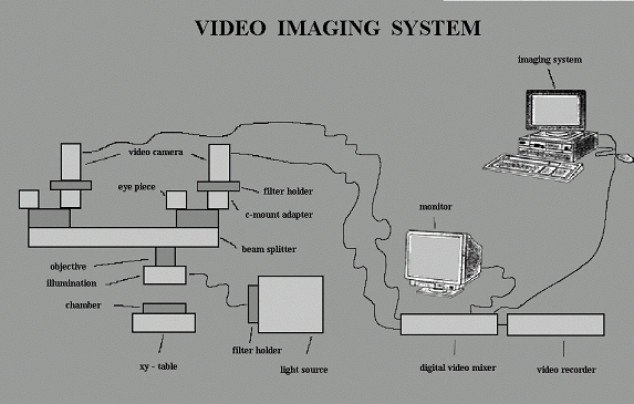

Figure 1B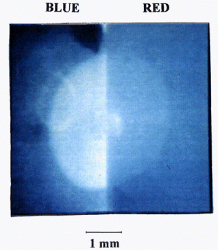

In figure 1A the setup for recording of SDs is shown. It consists of binocular microscope, which is mounted above a stepper-motor driven X-Y table. On the X-Y table Peltier elements are mounted for temperature control, on the top of them is a holder for the Petri dish. The perfusion of the solution in the dish is made with a peristaltic pump. In each of the visual pathways of the binocular microscope, beam splitters are mounted which are equipped with C-mount adapters. To these C-mount adapters, a variety of optical recording devices can be mounted. The illumination is made with a 150 W quartz-halogen lamp through a ring-light . In figure 1B a propagating wave is shown as seen by the two cameras, each with an optical filter in front. Note that the red scatter signal is brighter at the center or the origin of the wave, i.e. the stimulated region, in the rest of the wave, the blue scatter is stronger and more uniform than the red one.

Figure 2.

Figure 2 animation.

In order to demonstrate the changes in the intrinsic optical signal at the critical transition from quiescence to propagating wave, we recorded the stimulated region with the highest spatial resolution possible in our system (5 microns/pixel) using two cameras (see figure 1B). In front of each camera, an optical filter was positioned centered at 625 and 425 nm respectively, with a bandwidth of 20 nm. The total area under each camera was 750 m m2 .

In figures 2 and 3 we show the IOS at the critical transition in space-time plots. They were constructed the following way: the brightness of six consecutive frames (2 mm2 total area) were averaged pixel by pixel and them two successive averages were subtracted from each other. The temporal resolution in these difference frames is 240 msec. A total of 20 resultant frames were obtained from 600 msec to 4.8 seconds after the stimulus, just at the transition to propagation.

The red scatter brightness (figure 2) fluctuated in time-space, waxing and waning three times before the final amplification at the critical transition. The fluctuations in brightness tend to form ring in the fifth, thirteenth and finally, at the seventeenth difference frames. The sequence of the 19 difference frames is seen on the animation aside the figure.

Figure 3.

Figure 3 animation.

The blue scatter signal behavior is shown in figure 4. In order to see the slow ramp faction of its growth, we made differences from consecutive frames that were 1.5 seconds apart in time. Note that the growth is both in space and in intensity of the differences. Also that the process begins discrete in space and the spatial distribution differs in the red and the blue scatter of light.

This page was created and is maintained by João E. Kögler Jr.